Gradient Descent Methods Play a Critical Role in Machine Learning — Here’s How They Work

Introducing Gradient Descent, the Core of Most Machine Learning Algorithms

In our previous blog post, we provided an in-depth primer on linear algebra concepts and explained how to build a supervised learning algorithm. As part of this discussion, we reviewed linear models where our hypothesis set was composed of linear functions of the form

h_w(x) = = w₀ + w₁x₁ + w₂x₂ + … + w_dx_d

We also derived an analytic solution for w = (w₀, w₁, …, w_d) using the (x, y) values in our data set D. We determined that

w=(X^T X)^-1 X^T X y

where X is the matrix in which the row vectors are the x values from the elements of D, and y is the vector of the y values from the elements of D.

However, it’s not always possible or practical to perform this calculation. For example, the matrix X^T X might be singular or our data set might be too large to execute computations in a reasonable amount of time. In these cases, we can use an iterative approach.

Recall that the purpose of our analysis is to minimize error in the following function:

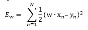
We accomplish this by computing the gradient of this function and finding a vector (w) that makes the gradient zero. But we can also take advantage of the fact that the gradient of a function at any given point is a vector that points in the function’s direction of steepest ascent — that is, the direction in which the value of the function increases fastest as we move away from that point.

Once we know the direction of steepest ascent, we can move in the opposite direction, and we’ll be moving in the direction of steepest descent. This is convenient, since if we keep moving along the negative gradient, we should eventually reach a minimal value.

This is exactly how the batch gradient descent algorithm works. The algorithm starts with an initial value of w, such as w = 0. Then, at each iteration, it computes the gradient ∇E_w and takes a small step along the negative of that gradient.

More precisely, given a “step size” α ϵ ℝ, at each iteration, we compute w  ⃪  w – α∇E_w until the change in w is small enough that we can feel confident that we’re at or near a minimal value of E_w.

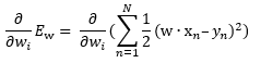
Let’s start by computing ∇E_w. This is a vector, and the i^th component of this vector comes from the partial derivative

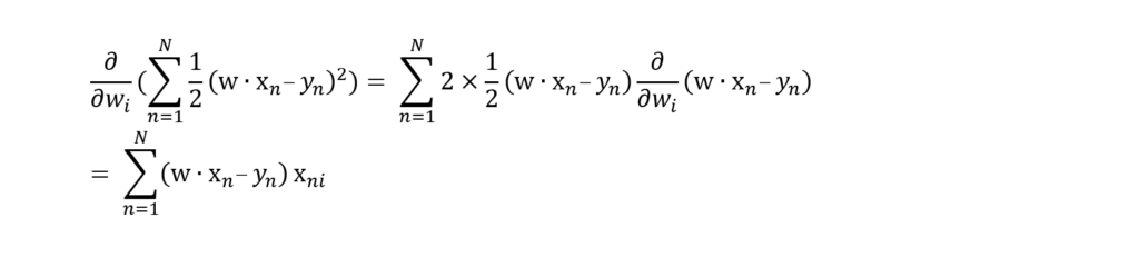
We can compute this partial derivative using the chain rule

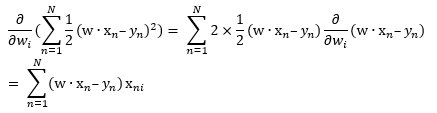
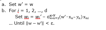
where x_ni denotes the i^th component of the vector x_n. So, our batch gradient descent algorithm looks like this:

1. Choose positive step size α ϵ ℝ and small positive ε ϵ ℝ. (For example, α = 0.01 and ε = 0.000001.)
2. Set w = (w₀, w₁, …, w_d) = (0, 0, …, 0)
3. Repeat …
   

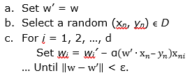
For very large data sets, this can still prove impractical since we must compute  for every iteration, which can be troublesome for very large N. In this case, we can use a variation of the algorithm known as stochastic gradient descent. In each step of this variation, we use only one data point instead of the entire data set. Then, step three of our algorithm becomes

1. Repeat …
   

This solution reduces the number of computations required in each iteration.

However, the trade-off is that we’re no longer following the gradient vector. Instead, we’re following a vector that is close to it. This means we’ll likely need many more iterations before we arrive at a minimal value, though we’ll make fewer computations on each iteration. And in some cases, we might not find a minimal value at all, so we’ll need to account for that issue in our overall solution.

The gradient descent methods described above work well for regression problems, where we’re trying to find a real-valued y. Another variation of gradient descent involves neural networks.

Unlike regression problems, selection problems involve trying to select a value of y from a discrete set instead of looking for a real-valued y. Gradient descent is utilized in selection problems as well, which is why it’s a must-know algorithm when working with machine learning. To make sure you don’t miss our next post about machine learning, check back on our site in the coming weeks or contact us and let us know you want to start receiving our exclusive newsletter.

Stratus Innovations Group: Turning Complex Machine Learning Concepts Into Real Business Solutions

The mathematical principles behind machine learning algorithms are fascinating, but you don’t need to understand every detail of them to realize the business benefits of machine learning — that’s why our team of experts is here. Stratus Innovations Group can help you develop a custom cloud-based solution that addresses your business’ unique needs and employs machine learning to improve maintenance routines, reporting, and other critical functions of your business.

To learn more about how Stratus Innovations can help your company become more profitable and efficient, call us at 844-561-6721 or fill out our quick and easy online contact form. We’ll help you bring the power of the cloud to your operations!